Chapter 3 Class 12 Physics Current Electricity Notes

Here, we have provided Class 12 Physics current electricity notes. These are very important for students of NCERT and CBSE boards.

Current Electricity

The branch of physics, which deals with the charges in motion and the phenomenon associated with such a flow is called Current Electricity.

Electric Current

An electric current is said to be existing through a section of a conductor if there is a flow of charge through that section of the conductor in a definite direction.

In order to maintain the flow of a charge in a conductor, a potential difference must be maintained across the ends of the conductor.

Mathematically, current is represented as the rate of flow of charge through a section of a conductor. The instantaneous rate of flow of charge with respect to time is:

\[I = \frac{dq}{dt}\]

Where \(dq\) is the amount of charge, and \(dt\) is the time interval.

Direction of Electric Current

The direction of current in a closed circuit is taken to be the same as the direction of flow of positive charge. The current in such a direction is said to be a conventional current.

However, the flow of electrons is opposite to that of the conventional current. The current due to the flow of electrons in a circuit is called electronic current.

Units

Also Check: Class 9 Science Floatation Notes

Electric current is one of the 7 basic physical quantities in physics. The SI unit of electric current is coulomb/second, which is named as ampere.

Current in a conductor is said to be one ampere if a charge of one coulomb crosses a section of a conductor during the time interval of one second.

\[1 milliampere (1 \, \text{mA}) = (10^{-3} \, \text{A})\]

Electric Current as a Scalar Quantity

Although electric current in a circuit represents the direction of flow of charge with a certain magnitude, it does not qualify to be a vector quantity.

It is due to the reason that current fails to obey the laws of vector addition. Electric currents in a circuit are added as scalars and not as vectors.

Types of Electric Current

There may be two kinds of electric current set up in a circuit on the basis of variation with respect to time:

1. Steady Current: An electric current is said to be a steady current or direct current (DC) if it does not change its magnitude and direction with time. Equal quantities of charge pass through a section of the conductor during equal intervals of time. Steady current is given by:

\[I = \frac{q}{t}\]

2. Varying Current: An electric current is said to be varying current if its direction, magnitude, or both show a change with respect to time. It is described by the instantaneous values in a circuit given as:

\[I = \frac{dq}{dt}\]

3. Alternating Current: It is a special kind of varying current, which changes continuously in magnitude and periodically in direction. The variation of such a current with time is represented by sine or cosine function.

Current in a Metallic Conductor

The structure of most pure metals is seen to be crystalline. The atoms are placed very close to each other with a density of the order of about \(10^{28}\) atoms/ \(m^3 \).

The atoms are in continuous vibratory motion even at room temperature. Since metals are rich in electrons, and under certain conditions, some become free, they are called free electrons. These free electrons leave behind positive ions in the crystal.

The free electrons can move through the inter-atomic spaces and jump from one atom to another. Hence, they constitute a mobile charge.

In the absence of an electric field, the free electrons move at random in all possible directions. Their number is of the order of \(10^{28}\) electrons per cubic meter.

Their random velocity at room temperature is of the order of \(10^6 \, \text{m/s}\), but the net velocity of the free electrons in the absence of an external field is zero.

Drift Velocity and its Expression

The free electrons in a metallic conductor are always in random motion when no electric field is applied.

Consider a hypothetical plane passing through a conductor; the number of electrons passing through it from left to right will be equal to those crossing in the opposite direction. Thus, the net flow of charge through this plane is zero.

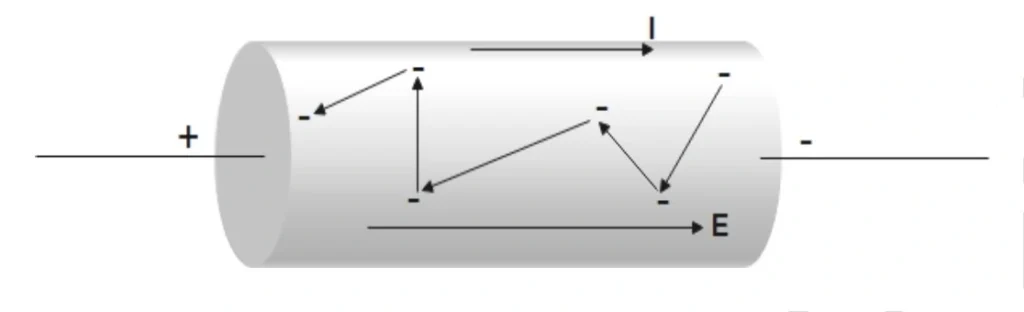
If the ends of the conductor are connected to a battery, an electric field will be set up at every point within the conductor. The force acting on the electron is given by:

\[
\mathbf{F} = -e \mathbf{E} \tag{1}
\]

The negative sign indicates that the direction of the force on the electron is opposite to the direction of the electric field.

The acceleration produced in the electron is:

\[
\mathbf{a} = \frac{\mathbf{F}}{m} = \frac{-e \mathbf{E}}{m} \tag{2}
\]

The accelerated electron gains an extra velocity, but this extra velocity is destroyed at each collision. This means that the average initial velocity of the electron is zero:

\[
U_{\text{avg}} = \frac{U_1 + U_2 + U_3 + \dots + U_n}{n} = 0
\]

So, the net result is that the electron acquires a slow drift velocity \((V_d)\) in the direction opposite to that of the electric field \((\mathbf{E})\).

Using the equations of motion for each electron, we have:

\[
V_d = U_{\text{avg}} + \mathbf{a} t
\]

Let the velocities in the presence of the electric field be \(V_1, V_2, V_3, \dots, V_n\).

For the average velocity:

\[
V_d = \frac{V_1 + V_2 + V_3 + \dots + V_n}{n}
\]

\[ \scriptsize \implies V_d = \frac{U_1 + a t + U_2 + a t + \dots + U_n + a t}{n} \]

Simplifying,

\[
V_d = 0 + a t = a t \tag{3}
\]

Here, (t) is replaced by (𝜏), which represents the mean time between two successive collisions of the electron with fixed positive ions.

The time (𝜏) is known as relaxation time, and the distance traveled between successive collisions is known as the free path.

Substituting (a) from equation (2) into (3):

\[
V_d = \frac{-e E \tau}{m} \tag{4}
\]

Hence, drift velocity is the velocity with which the electrons are drifted through the conductor under the influence of an external field.

Relation Between Drift Velocity and Electric Current

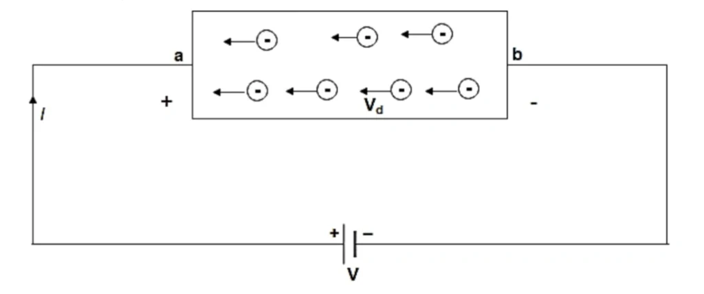
Let us consider a conductor (AB) of length \(l\). Let \(V\) be the potential difference between (A) and (B). Then the electric field is:

\[
E = \frac{V}{l} \tag{1}
\]

Let \(A\) be the area of cross-section of the conductor, \(V_d\) be the magnitude of the drift velocity of electrons, and (n) be the number of electrons per unit volume of the conductor.

The total number of electrons in the conductor is \(n \times (\text{Volume of conductor})\)

\[
\implies \text{Total electrons} = n \cdot A \cdot l
\]

If (e) is the charge on each electron, the total charge in the conductor is given by;

\[
q = n \cdot A \cdot l \cdot e \tag{2}
\]

Now the time taken by the electrons to cover the length (l) moving with velocity \(V_d\) is:

\[
t = \frac{l}{V_d} \tag{3}
\]

By definition of electric current:

\[
I = \frac{q}{t}
\]

Substituting (q) from (2) and (t) from (3) in the above equation, we get

\[
I = \frac{n \cdot A \cdot l \cdot e}{l / V_d}
\]

Simplifying:

\[
I = n e A V_d \tag{4}
\]

This is the required relation between drift velocity and current.

Mobility

• It is drift velocity per unit electric field applied across the ends of the conductor.
• Mobility is represented by (μ), and is given by;

\[
\mu = \frac{V_d}{E} \tag{1}
\]

• The SI unit of mobility is m²V^-1s^-1

Now we know that \( V_d = \frac{eE\tau}{m} \),

Substituting it in the equation (1), we get;

\[
\mu = \frac{e\tau}{m}
\]

Ohm’s Law (VI Relation)

Statement: the current flowing through a conductor is proportional to the potential difference across its ends, provided the physical conditions of the conductor remain unchanged.

If \( V \) is the potential difference between the ends of a conductor and \( I \) is the current flowing through it, then:

\[
V \propto I \quad \text{or} \quad V = IR
\]

Here, \( R \) is the constant of proportionality and is called the resistance of the conductor.

Resistance

1. It is the net opposition offered to the passage of current through a conductor.
2. It originates due to collisions between positive fixed ions and electrons in the crystal.
3. For a given conductor, resistance is constant at a given temperature.

Derivation of Ohm’s Law

The current \( I \) set up in a conductor is given as:

\[
I = n e A V_d \tag{1}
\]

Here:

• \(n\) is the density of electrons in the conductor,
• \(A\) is the area of cross-section, and
• \(V_d\) is the drift velocity.

From the expression for drift velocity,

\[
V_d = \frac{eE\tau}{m} \tag{2}
\]
Substitute \( V_d \) from (2) into (1):

\[
I = n e A \cdot \frac{eE\tau}{m} = \frac{n e^2 A \tau E}{m} \tag{3}
\]

The electric field \(E\) in the conductor is related to the potential difference \(V\) as:

\[
E = \frac{V}{l} \tag{4}
\]

Substitute \(E\) from (4) into (3), we can write

\[
I = \frac{n e^2 A \tau}{m} \cdot \frac{V}{l} = \frac{n e^2 A \tau}{m l} \cdot V \tag{5}
\]

Compare this with \( I = \frac{V}{R} \), we can write;

\[
R = \frac{m l}{n e^2 \tau A} \tag{6}
\]

Resistivity (ρ)

1. The factor \( \frac{m}{n e^2 \tau} \) is called the resistivity of a conductor.
2. It is constant for a given conductor.
3. It is denoted by \(rho\), and therefore we can write;

\[
\therefore \rho = \frac{m}{n e^2 \tau}
\]

Using this in equation (6) above, we get;

\[
R = \rho \cdot \frac{l}{A}
\]

Laws of Resistance

1. Resistance \(R\) is directly proportional to the length of the conductor \(l\);

\[
\implies R \propto l
\]

2. Resistance \(R\) is inversely proportional to the area of cross-section \(A\);

\[
\implies R \propto \frac{1}{A}
\]

Conductance and Conductivity

The reciprocal of resistance is called conductance (G)

\[
\therefore G = \frac{1}{R},
\]

• The unit of ( G ) is (ohm)^-1 or Siemens (S).

The reciprocal of resistivity is called conductivity (σ);

\[ \therefore \sigma = \frac{1}{\rho}\]

• The unit of (σ) is Sm^-1.

Combination of Resistors

Resistors in Series

Two or more resistors are said to be connected in series if the same current flows through each resistor when a potential difference is applied across the combination. However, the potential difference across each resistor may be different.

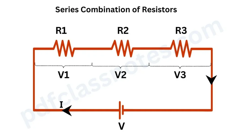
As shown in the figure, three resistors \(R_1, R_2, R_3\) are connected in series. Let \(V\) be the potential difference applied across the combination using the battery.

In series combination, the same current (I) will pass through each resistor.

Let \(V_1, V_2, V_3\) be the potential differences across \(R_1, R_2, R_3\) respectively.

Now applying Ohm’s law separately to all the resistors, we can write;

\[
V_1 = IR_1, \quad V_2 = IR_2, \quad V_3 = IR_3
\]

Now \(V = V_1 + V_2 + V_3 \)

Using values of \(V_1, V_2, V_3\) we can write that

\[
V = I R_1 + I R_2 + I R_3
\]

\[ V = I (R_1 + R_2 + R_3) \tag{1}\]

If \(R_s\) is the equivalent resistance of the given combination, then:

\[
V = I R_s \tag{2}
\]

From the equations (1) and (2), we can write;

\[
R_s = R_1 + R_2 + R_3
\]

Thus, the equivalent resistance of resistors in series is the sum of the individual resistances. For ( n ) resistors, this is:

\[
R_s = R_1 + R_2 + \dots + R_n
\]

Resistors in Parallel

Two or more resistors are said to be connected in parallel if the potential difference across each of them is the same and is equal to the applied potential difference across the combination.

As shown in the figure, three resistors \(R_1, R_2, R_3\) are connected in parallel. Let \(V\) be the potential difference applied across the combination using a battery.

Let \(I\) be the total current in the circuit and \(I_1, I_2, I_3\) the currents through \(R_1, R_2, R_3\) respectively.

From Kirchhoff’s current law:

\[
I = I_1 + I_2 + I_3 \tag{3}
\]

Since the potential difference across each resistor is \(V\).

\[
I_1 = \frac{V}{R_1}, \quad I_2 = \frac{V}{R_2}, \quad I_3 = \frac{V}{R_3}
\]

Substituting these into the equation (3), we get:

\[
I = \frac{V}{R_1} + \frac{V}{R_2} + \frac{V}{R_3} \tag{4}
\]

If \(R_p\) is the equivalent resistance, then:

\[
I = \frac{V}{R_p} \tag{5}
\]

Comparing equations (4) and (5, we get;

\[
\frac{1}{R_p} = \frac{1}{R_1} + \frac{1}{R_2} + \frac{1}{R_3}
\]

For (n) resistors in parallel, the result is generalized as:

\[
\frac{1}{R_p} = \frac{1}{R_1} + \frac{1}{R_2} + \dots + \frac{1}{R_n}
\]

Temperature Dependence of Resistivity

The temperature dependence of resistivity can be qualitatively explained with the expression of resistivity in terms of average relaxation time,

\[
\rho = \frac{m}{n e^2 \tau} \quad = \quad \frac{1}{\sigma}
\]

Where:

• (m) = mass of electron,
• (σ) = conductivity,
• (n) = number of free electrons,
• (e) = charge of electron,
• (𝜏) = relaxation time.

As \(m, n, e\) are constants for different conductors of the same material:

\[
\frac{1}{\sigma} = \rho \propto \frac{1}{\tau}
\]

From this expression, it is clear that resistivity is inversely proportional to the average relaxation time (𝜏) and number density of electrons (n).

In the case of conductors, with an increase in temperature, the frequency of collisions of electrons or ions increases, which reduces the average relaxation time (𝜏) and thus the resistivity increases with the rise in temperature.

However, the number density of free electrons (n) does not change with the change in temperature. As (R ∝ ρ), resistance also increases with the rise in temperature.

The relation between temperature and resistivity for copper and metals, in general, is fairly linear over a broad temperature range.

In general, we can say that for conductors, the resistivity increases with the increase in temperature, and a relation that explains this increase mathematically is:

\[
\rho – \rho_0 = \rho_0 \alpha (T – T_0) \quad \text{—- (2)}
\]

Where (T₀) is a selected reference temperature, and (ρ₀) is the resistivity at that temperature, usually:
(T₀ = 293K) (room temperature), for which (ρ₀= 1.69 x 10^-8 Ω m) for copper.
(ρ) is the resistivity of the material of a conductor at (T°C) or (T K).

It does not matter whether we use the Celsius scale or the Kelvin scale because the temperature difference on these scales is identical. The quantity (α) is called the temperature coefficient of resistivity, and its unit is per degree.

(α) may be defined as the ratio of the increase in resistivity per degree rise in temperature to its resistivity at (T°C).

From eq. (2), we have:

\[
\rho – \rho_0 = \alpha \rho_0 (T – T_0)
\]

\[
\alpha = \frac{\rho – \rho_0}{\rho_0 (T – T_0)} = \frac{\Delta \rho}{\rho_0 \Delta T}
\]

The value of (α) can be determined through experiments. For copper, the value of (α) is found to be (0.004 per degree).

For metals, the value of (α) is positive and lies between (10^-2) to (10^-4°C^-1).

ALLOYS:

In the case of alloys, the resistivity is large, and it has a very weak dependence on temperature. For example, Nichrome, Manganin, and Constantin have a resistance that is 30 to 40 times as that of pure copper for the same dimensions, but their temperature coefficient is very small:

\[
\alpha = 0.00001 \, \text{per degree}.
\]
That is why alloys are used for making standard resistances.

SEMICONDUCTORS:

1. The semiconductors like Si and Ge show an opposite trend.
2. The resistivity of semiconductors generally decreases with the increase in temperature.
3. Due to the rise in temperature, there is an increase in the concentration of charge carriers, and hence conductivity increases.
4. The semiconductors show a negative temperature coefficient of resistance.

The temperature dependence of resistivity of semiconductors and insulators is given by:

\[
\rho = \rho_0 e^{\frac{E_g}{kT}}
\]

Where:

• \(k\): Boltzmann constant,
• \(E_g\): Energy gap between the valence band and conduction band,
• \(T\): Absolute temperature.

Internal Resistance of a Cell & its EMF

A cell is a device used to maintain a steady current in an electric circuit.

Internal Resistance of a Cell is defined as the resistance offered by the electrolyte and the electrodes of a cell when the current flows through it.

Internal resistance of a cell is denoted by (r) and depends on:

1. Distance between the electrodes.
2. The nature and concentration of the electrolyte.
3. The area of electrodes immersed in the electrolyte.

The agency or device used to produce the EMF in a circuit is known as the source of EMF. The source of the EMF may use mechanical, chemical, light, or heat energy to provide electrical energy in return. Examples include batteries, generators, and phototubes, which can act as sources of EMF in an electrical circuit.

The Electromotive Force (E.M.F) of a cell may be defined as the potential difference between the terminals of a battery (treated as a cell) when no current is drawn from it. The SI unit of the EMF is Volt (V). EMF is denoted by (ε).

It may also be defined as the total work done in carrying a unit positive charge once around the complete circuit, including the cell, and is given by:

\[
\epsilon = \frac{dw}{dq}
\]

The unit of (ε) is Joule/Coulomb or Volt.

Difference Between Potential Difference and EMF of a Source

If a battery maintains a potential difference of 1V between its terminals, it is not always true that the EMF of the battery is 1V. This is true only under specific conditions.

A battery converts chemical energy into electrical energy. Practically, it is not possible to obtain an ideal or perfect battery. Some energy is always lost inside the battery.

Therefore, there is always some internal resistance shown by the battery. This internal resistance behaves in the same way as an external resistance.

The figure shows a battery with internal resistance (r) and external resistance (R) connected in the circuit.

The terminal voltage is:

\[
V = V_A – V_B = \epsilon – Ir
\]

Thus:

\[
V = \epsilon – Ir
\]

The terminal voltage equals EMF under the following conditions:
a) (I = 0), when no current is drawn (open circuit).
b) (r = 0), the internal resistance of the battery is zero.

According to Kirchhoff’s second law:

\[
\epsilon – Ir – IR = 0
\]

Thus:

\[
\epsilon = I(r + R)
\]

or:

\[
I = \frac{\epsilon}{r + R}
\]

This equation gives the current in the circuit.

Combination of Cells

Cells can be combined in different ways to get the desired potential difference and a desired current for a desired period through the load. There are three types of groupings of the cells:

1) Cells in Series

The cells are said to be in series grouping if the positive terminal of one cell is connected to the negative terminal of the second cell, whose positive terminal is connected to the negative terminal of the third cell, and so on. The free ends of the first and last terminal are connected with the external resistor.

Let \(n\) identical cells be connected in series, each of EMF \(\epsilon\) and internal resistance \(r\). Let \(R\) be the resistance of the external resistor. Since the internal resistances of the cells are connected in series:

Total internal resistance of (n) cells= \(nr\)

Total resistance of the circuit = \(nr + R\)

Effective EMF of (n) cells = \( n\epsilon \)

The current in the resistance (R) is given by;

\[ I = \frac{n\epsilon}{nr + R} \]

Special Cases:

(1) If \(R >> nr\), \( I = \frac{n\epsilon}{R} \)

In this case, the current in the external resistance is (n) times the current due to a single cell.

(2) If \(R << nr\), \( I = \frac{\epsilon}{r} \)

In this case, the current in the external resistance is the same as that due to a single cell.

2) Cells in Parallel

The cells are said to be connected in parallel if the positive terminals of all the cells are wired together at one point (X) and their negative terminals at another point (Y). The external resistor \(R\) is connected between (X) and (Y) as shown.

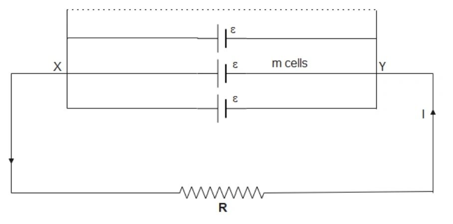
Let \(m\) identical cells be connected in parallel, each of EMF \(\epsilon\) and internal resistance \(r\). Let \(R\) be the resistance of the external resistor. The internal resistances of all the cells are connected in parallel, so the total internal resistance \(r_p\) is given by:

\[ \frac{1}{r_p} = \frac{1}{r} + \frac{1}{r} + \dots \, m \, \text{times} \]

Thus \(r_p = \frac{r}{m}\)

The external resistance \(R\) is connected in series with the internal resistance \(r_p\).

Total resistance in the circuit:

\[
R + \frac{r}{m}
\]

In parallel combinations of cells, the effective EMF in the circuit is equal to the EMF due to a single cell.

The current in resistance \(R\) is given by:

\[
I = \frac{\epsilon}{R + \frac{r}{m}}
\]

or:

\[
I = \frac{m\epsilon}{mR + r}
\]

Special Cases:

(1) If \(mR << r\), \( I = \frac{m\epsilon}{r} \)

(2) If \(r << mR\), \( I = \frac{\epsilon}{R} \)

In this case, the current in the external resistance is the same as due to a single cell.

3) Cells in Mixed Grouping

The cells are said to be in mixed grouping if a number of rows of cells are connected in parallel to each other as shown in the figure below:

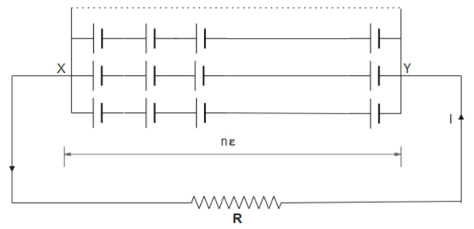
Let us consider that there are \(n\) cells in series in one row and \(m\) rows of cells in parallel. All the cells are identical with EMF \(\epsilon\) and internal resistance \(r\) each.

The total internal resistance of each row: \(nr\)

The total EMF of each row = \(n\epsilon\)

Since there are (m) rows of cells in parallel, the total internal resistance \(r_p\) of all the cells is given by:

\[ \frac{1}{r_p} = \frac{1}{nr} + \frac{1}{nr} + \dots \, \text{upto (m) times} \]

Thus:

\[ \frac{1}{r_p} = \frac{m}{nr}, \quad \text{or} \quad r_p = \frac{nr}{m} \]

The parallel combination of cells does not affect the EMF of the cells but only increases the size of the electrodes.

Total resistance in the circuit = \( R + \frac{nr}{m}\)

Now, the current in the external resistance is given by:

\[
I = \frac{n\epsilon}{R + \frac{nr}{m}}
\]

or \[I = \frac{mn\epsilon}{mR + nr} \]

We can use the concept of maxima and minima of a function to find the condition for the current to be maximum in the circuit. Mathematically, it can be shown that \(I\) will be maximum if:

\[
mR = nr \quad \text{or } \quad R = n \times \frac{r}{m}.
\]

Thus, for \(I\) to be maximum in a mixed grouping of cells, the value of external resistance should be equal to the total internal resistance of all the cells.

Special Cases:

• If \(m = 1\), the mixed grouping reduces to the case of cells in series.
• If \(n = 1\), the mixed grouping reduces to the case of cells in parallel.

---

Kirchhoff’s Laws

Sometimes it becomes very difficult to solve circuits using Ohm’s law. In such cases we use Kirchhoff’s laws.

To understand these rules, we define two terms:

1. Branch Point: A branch point is a point in the circuit where three or more conductors are joined together.
2. Loop: A loop is a closed path in a circuit along which the current flows.

Kirchhoff’s First Law (Current Law/Junction Rule)

“The sum of all the currents entering any junction point is equal to the sum of all the currents leaving that junction point.

In other words: “The algebraic sum of all the currents flowing towards a branch point is zero.”

\[ \sum I_j = 0 \]

Kirchhoff’s first law is based on the law of conservation of charge. The charge cannot accumulate at a point in the circuit.

Example: Consider the branch point in a circuit as shown in the figure. Kirchhoff’s junction rule gives the relation:

Current leaving the branch point = Current entering the branch point.

\[
\text{That is } I_1 + I_4 = I_2 + I_3 + I_5
\]

Or:

\[
I_1 – I_2 – I_3 + I_4 – I_5 = 0 \quad \text{(i.e., \(\sum I_j = 0)\)}.
\]

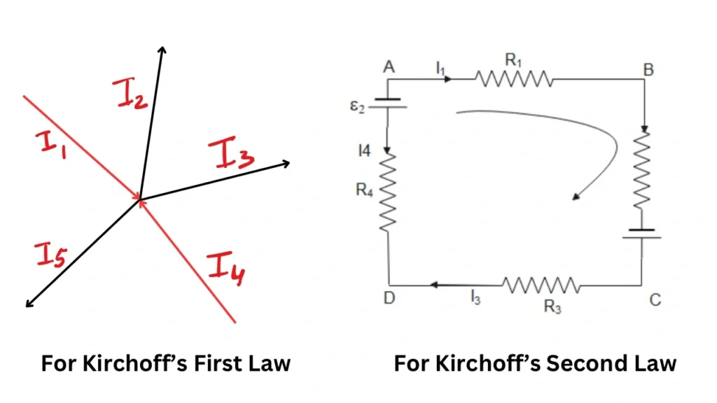
Kirchhoff’s Second Law (Loop Rule/Voltage Law)

It states:“In a closed loop, the sum of changes in electric potential of a moving charge around the complete circuit must be zero.”

Kirchhoff’s second rule is a direct outcome of the law of conservation of energy.

In other words: “The algebraic sum of all the potential differences along a closed loop in a circuit is zero.”

\[ \text{That is }\sum V = 0 \]

Rules for Applying Kirchhoff’s Laws:

(1) In Junction Rule:

• The current flowing towards the junction is taken as positive, and the current flowing away from the junction is taken as negative.

(2) In Loop Rule:

• The EMF of the cell is taken as negative if one moves in the direction of increasing potential difference, and vice versa.
• The product of resistance and current in an arm is taken positive if the direction of current in that arm is the same as one moves in a closed path, and vice versa.

Example:
The figure above shows a closed loop (ABCDEF) of a circuit.

As we start from (A) and go along the loop clockwise to reach the same point (A), we have:

\[
I_1 R_1 + I_2 R_2 – \epsilon_1 + I_3 R_3 – I_4 R_4 + \epsilon_2 = 0
\]

Applications of Kirchhoff’s Laws

Wheatstone Bridge

Wheatstone, in 1843, designed a network of four resistances that can accurately measure the resistance of a given resistor. This arrangement is called a Wheatstone Bridge. It is a resistance network used in the laboratory for rapid and precise measurements of resistance.

Construction:

A Wheatstone Bridge consists of four resistors \(R_1, R_2, R_3 and R_4\) arranged to form a quadrilateral (ABCD).

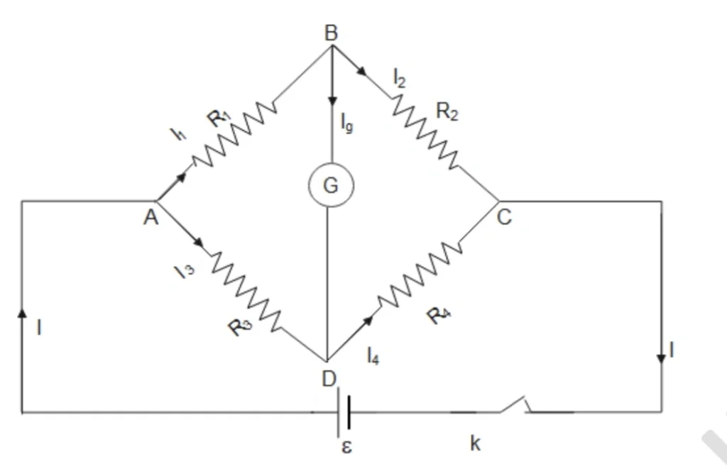
A galvanometer (G) is applied across points (B) and (D), as shown. A battery is placed in the circuit between ends (A) and (C) and is provided with a key (K₁). Another key is provided in the arm of the galvanometer (denoted (K₂) in the figure).

Principle:

The working of a Wheatstone Bridge is based on the following principle:
“If the resistances \(R_1, R_2, R_3 and R_4\) forming the Wheatstone Bridge are adjusted so that there is no current in the galvanometer (I_g = 0), the bridge is said to be balanced. Under such conditions, the resistances are in the following proportion:”

\[
\frac{R_1}{R_2} = \frac{R_3}{R_4}
\]

Proof:

Let the battery cause current \(I\) to flow through point (A). At point (A), the current splits into parts \(I_1\) and \(I_3\), flowing through arms (AB) and (AD), respectively.

Applying Kirchhoff’s Junction Rule at point (B), we have \(I_1 = I_2 + I_g\)

If the bridge is balanced, \(I_g= 0\), and \(I_1 = I_2\)

Applying Kirchhoff’s Junction Rule at point (D), we have \(I_3 + I_g = I_4\)

If \(I_g = 0\), then \(I_3 = I_4\)

Thus, under balanced conditions:

\[
I_1 = I_2 \quad \text{and} \quad I_3 = I_4 \quad \text{— (1)}
\]

Applying Kirchhoff’s Voltage Law to the loop (ABDA):

\[
I_1 R_1 + I_g G – I_3 R_3 = 0
\]

Substitute \(I_g = 0\):

\[
I_1 R_1 = I_3 R_3 \quad \text{— (2)}
\]

Applying Kirchhoff’s Voltage Law to the loop (ABCDA):

\[
I_1 R_1 + I_2 R_2 – I_4 R_4 – I_3 R_3 = 0 \quad \text{— (3)}
\]

Using (2) in (3), we get:

\[
I_2 R_2 = I_4 R_4 \quad \text{— (4)}
\]

Dividing Equation (2) by Equation (4):

\[
\frac{I_1 R_1}{I_2 R_2} = \frac{I_3 R_3}{I_4 R_4}
\]

Using Equation (1):

\[
\frac{R_1}{R_2} = \frac{R_3}{R_4}
\]

Generally, \(R_4\) is an unknown resistance to be measured. Since \(R_1, R_2, R_3\) are known, \(R_4\) can be calculated by balancing the bridge.

The Wheatstone Bridge is available in many forms, two of which are The Post Office Box and The Meter Bridge.

Meter Bridge or Slide Wire Bridge

A Slide Wire Bridge is a modified form of a Wheatstone Bridge. It provides a convenient method of measuring low resistances in the laboratory.

Construction:

It consists of a wire (AC) made of constantan or manganin alloy, 1 meter in length, and of uniform cross-section. The wire is stretched between copper strips on a horizontal wooden board. A scale 1 meter long is fitted on the wooden board parallel to the wire.

There are two gaps provided between the copper strips. Across one gap, a resistance box (R) is connected, and across the other gap, the unknown resistance (X) is connected. A jockey (J) can slide on the bridge wire. One terminal of a sensitive galvanometer (G) is connected to the jockey (J), and the other terminal to point (D). A battery (E) is connected between terminals (A) and (B) through a one-way key.

Working:

To measure an unknown resistance (X), follow these steps:

1. Close the key and adjust the resistance box (R) for a suitable value.
2. Adjust the position of the jockey (J) on the wire so that when pressed on the wire, the galvanometer shows no deflection. Let this point be (B).
3. Measure the length (AJ = l). Then, the length (JB = 100 – l).

When the bridge is balanced:

\[
\frac{P}{Q} = \frac{R}{X}
\]

Here:

• \(P = l r\), the resistance of the length \(l\) of wire,
• \(Q = (100 – l) r\), the resistance of the length (\(100 – l)\) of wire,
• \(r\), the resistance per cm length of the wire.

Thus:

\[
\frac{l r}{(100 – l) r} = \frac{R}{X}
\]

\[
X = R \cdot \frac{(100 – l)}{l}
\]

By knowing \(l\) and \(R\), the unknown resistance (X) can be calculated.

POTENTIOMETER

It is an instrument used for the accurate measurement of an unknown EMF or a small potential difference.

Principle and Working

As shown in the diagram below, AB is a long wire of uniform resistance connected to a battery (ε₁).
(ε₁) is known as the auxiliary battery. (ε₁) maintains a current in the wire flowing from A to B. Let (ρ) be the fall of potential gradient:

\[
\rho = \frac{\varepsilon_1}{L} \quad \text{or} \quad \varepsilon_1 = L \cdot \rho
\]

The source with unknown EMF (ε₂ ) is connected with its positive terminal to the end A and other end to the wire through the jockey J.

As the jockey is moved from A to B, the potential difference between A and J keeps increasing. As soon as the potential difference between A and J becomes equal to (ε₂), the galvanometer shows no deflection. There is no current in the galvanometer wire.

Let (l₂ ) be the length of wire at zero deflection.

\[
\varepsilon_2 = l_2 \cdot \rho
\]

Thus, at zero deflection, ( ε) is directly proportional to (l) (where ( \rho ) is constant for a given wire).
It is important to note that (ε₂) can be balanced with a part of wire AB if ε₁ > ε₂.

The principle of the potentiometer thus states:

The EMF of a cell is directly proportional to the length of the wire for which the balance point is obtained.

Since no current is drawn from the source of EMF at the balance point, the potentiometer measures the actual or absolute EMF of the cell. This is a major advantage of the potentiometer over the voltmeter.

Comparison Between EMF of Two Cells Using a Potentiometer

Let us consider the cells with EMFs (ε₁) and (ε₂) to be compared with each other. Let (ε) be the EMF of the auxiliary battery in the circuit of the potentiometer.

It is important that the EMF (ε) must be greater than both (ε₁) and (ε₂). The positive terminals of ε, ε₁ and ε₂ are connected to point A.

Steps:

1. The two-way key is put into position 1 so that the cell (ε₁) is brought into the circuit. Let (l₁) be the length of the wire corresponding to the balance point for the cell (ε₁).
2. Similarly, let (l₂) be the length of the wire corresponding to the balance point for cell (ε₂).

From the principle of the potentiometer:

\[
\varepsilon_1 \propto l_1 \quad \text{and} \quad \varepsilon_2 \propto l_2
\]

Dividing the two equations:

\[
\frac{\varepsilon_1}{\varepsilon_2} = \frac{l_1}{l_2}
\]

Thus, the ratio of (ε₁) and (ε₂) is found by measuring (l₁) and (l₂) experimentally.

Determination of Internal Resistance of a Cell by Potentiometer

Let (ε) be the EMF of the cell whose internal resistance is to be determined and is connected in the potentiometer circuit as shown.

Steps:

Step 1: By closing key (K’), a suitable current is set up through the potentiometer wire AB with the help of rheostat (Rh).

Step 2: By adjusting the jockey along the wire AB at different points, the balance point is achieved where the galvanometer shows no deflection. Let this point be at (J), and let (AJ = l₁). The length (l₁) is noted. This step gives the value of (ε) as:

\[
\varepsilon = \rho \cdot l_1 \tag{1}
\]

Here, (ρ) is the potential gradient across the wire.

Step 3: Now the resistance (R) is brought into the circuit of the cell by closing the key (K). The resistance (R) will draw a finite current from the cell. Under this condition, the balance point is again achieved by adjusting the jockey.

Let the balance point be at (J₁), and let (AJ₁=l₂). The length (l₂) is noted down from the scale of the potentiometer. This step gives the potential difference (V) of the cell when the current is drawn by resistance (R):

\[
V = \rho \cdot l_2 \tag{2}
\]

Step 4: The relation between V, ε and internal resistance ( ) of the cell is:

\[
\varepsilon = V + I \cdot r
\]

Rearranging:

\[
r = \frac{\varepsilon – V}{I} \tag{3}
\]

Since ( I = V/R ), substituting this into equation (3), we get:

\[
r = \frac{\varepsilon – V}{V / R} \tag{4}
\]

Substituting the values of (ε) and (V) from equations (1) and (2):

\[
r = \frac{\rho \cdot l_1 – \rho \cdot l_2}{\rho \cdot l_2 / R}
\]

Simplifying further and we get;

\[
r = \left( \frac{l_1 – l_2}{l_2} \right) R
\]

Thus, the internal resistance of the cell is determined using the values of l_1, l₂ and R.

Also Check: Gravitation notes class 9 Physics

---

So, these were Class 12 Physics Current Electricity Notes for NCERT and CBSE students. We are sure that you have loved these notes.